6  Visualise and handle trees

6.1 Phylogeny handling and visualisation in R and Figtree

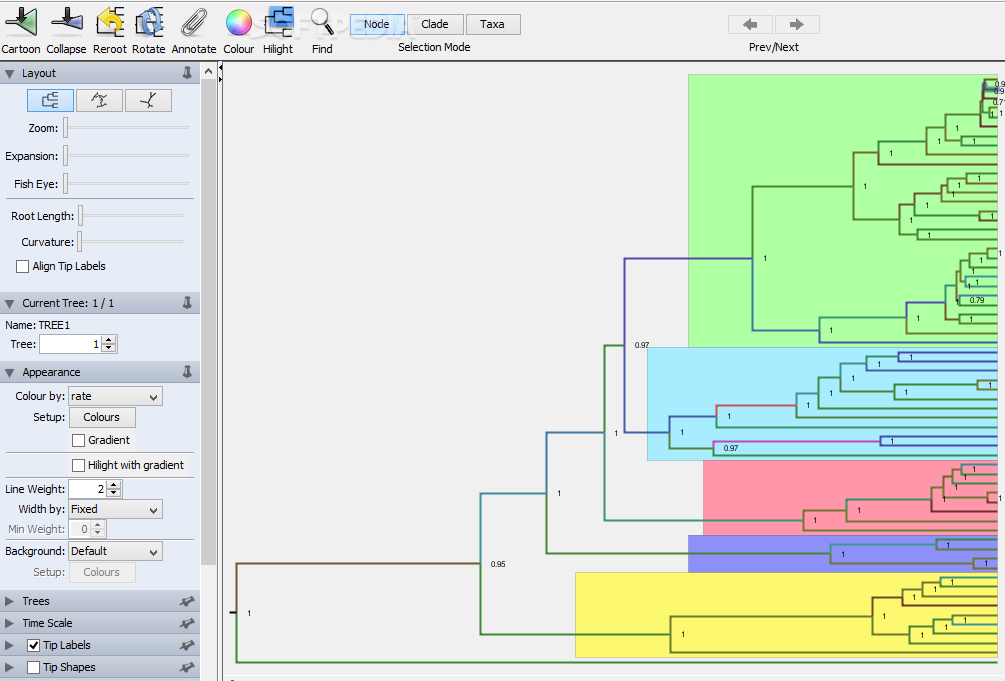
6.1.1 Open your maximum credibility tree in Figtree.

Here you can visualize the tree topology, the posterior probability of different nodes (support values) and the node ages. Explore the different visualisation options in the drop-down menus by trying out different settings.

A useful option is to select “Node labels” (left panel) and select display “Node ages” to see the ages of the nodes.

Or select display “posterior” to see the posterior distribution support values.

Play around with Figtree - this will be useful for tomorrow’s practical :)

6.1.2 Open R to load your tree

Now let’s explore some of the functions of R applied to phylogenies.

Welcome to R

First let’s clear your workspace, in case you have some saved objects there that may interfere with the practical

rm(list=ls())

Load the necessary packages to run the practical

library(ape)

Load the maximum clade credibility tree you produced in the Beast analysis. Here you need to change the path to the file to match the location on your computer

cyanistes<-read.nexus('Cyanistes.tre')

Let’s see what the cyanistes object is

cyanistes

Phylogenetic tree with 70 tips and 69 internal nodes.

Tip labels:
  Cyanistes_caeruleus_KY378741.1, Cyanistes_caeruleus_caeruleus_DQ474042.1, Cyanistes_caeruleus_caeruleus_KP759222.1, Cyanistes_caeruleus_calamensis_JF828080.1, Cyanistes_caeruleus_calamensis_KC202361.1, Cyanistes_caeruleus_calamensis_KP759197.1, ...

Rooted; includes branch lengths.

Let’s see what the tip labels are

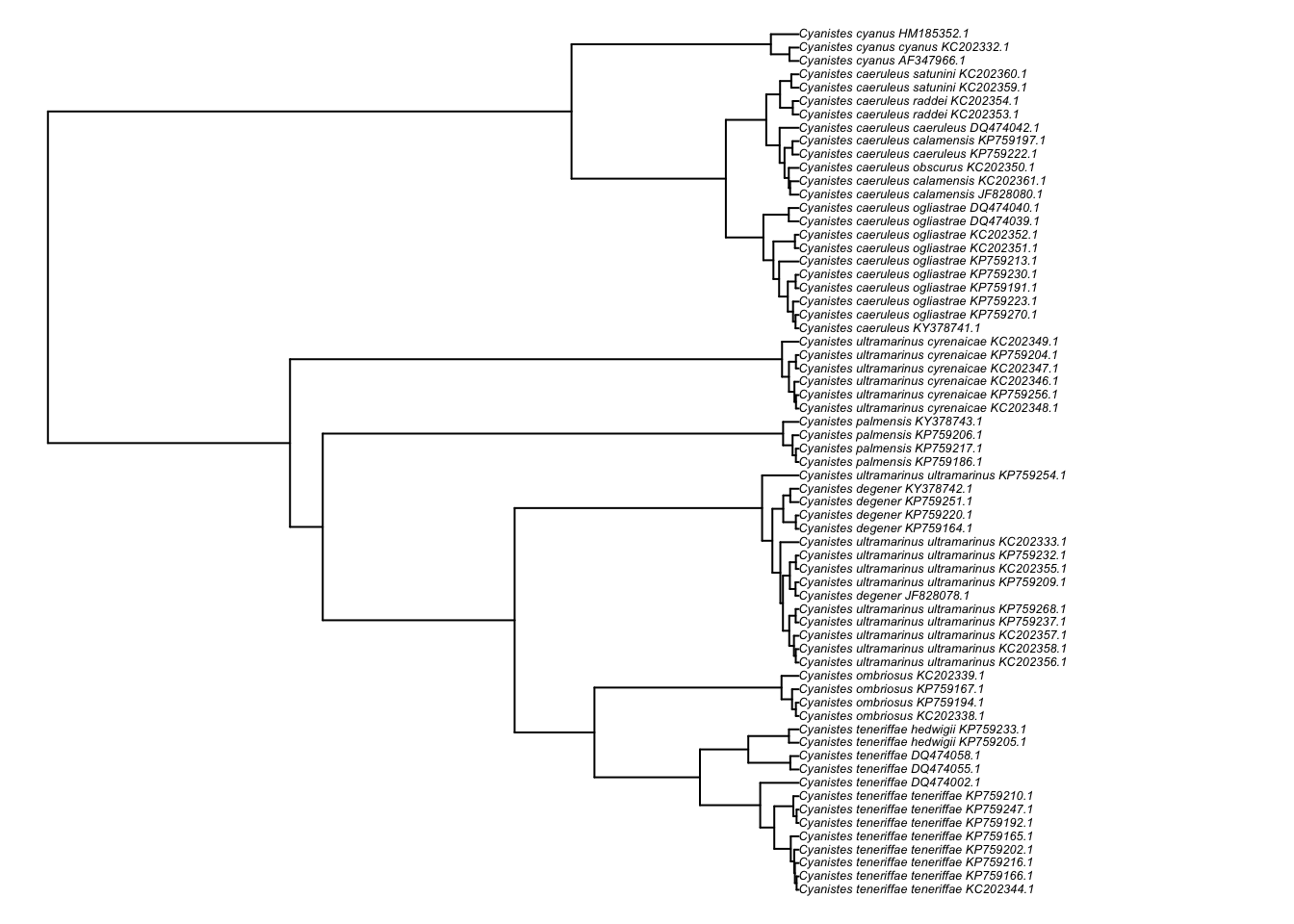
cyanistes$tip.label

Plot the phylogeny

plot(cyanistes)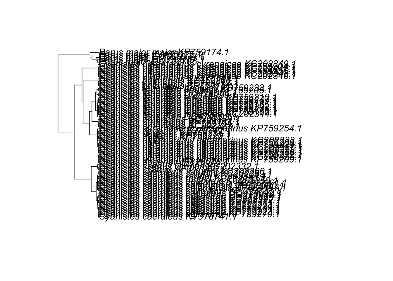

Looks a bit messy.

Plot with smaller tip labels

plot(cyanistes,cex=0.4)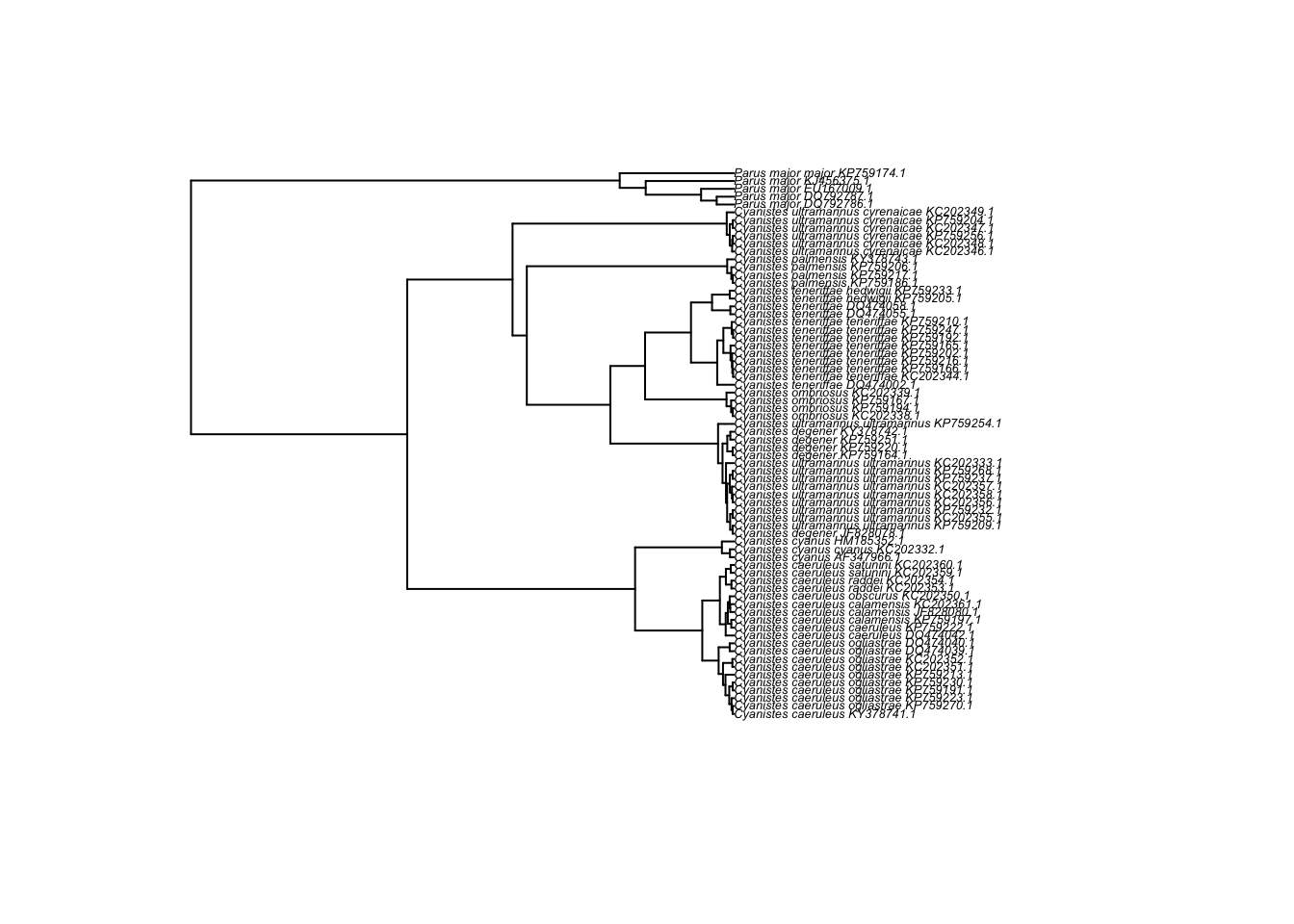

If the above still looks odd, try re-setting the margins of the R plot window, using par(mar = c(0, 0, 0, 0))

And a neater version, using the ladderize option (can you tell the difference?):

plot(ladderize(cyanistes),cex=0.4,no.margin=TRUE)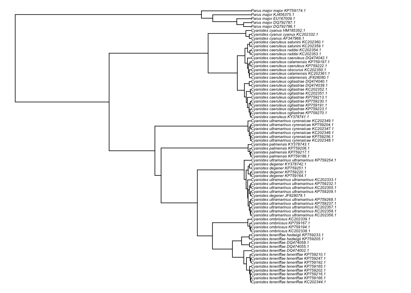

Check if the tree is ultrametric. This is essential for downstream analyses that rely on a dated tree.

is.ultrametric(cyanistes)

[1] TRUE

Plot the node labels

plot(ladderize(cyanistes),cex=0.4,no.margin=TRUE)
nodelabels(cex=0.3,frame='circle',bg='grey')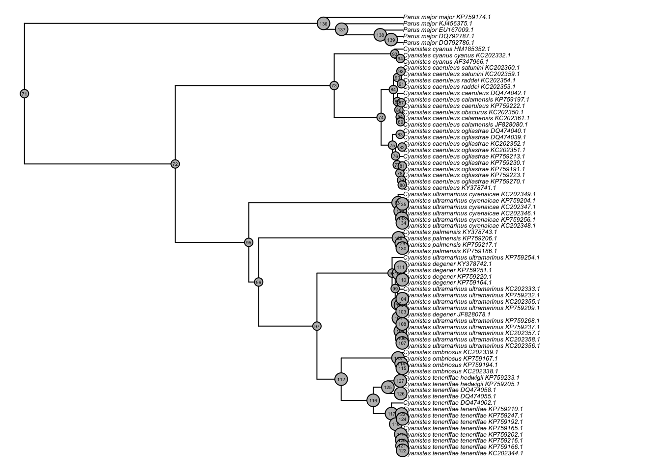

Plot as a fan.

plot(ladderize(cyanistes),type='fan',cex=0.3,no.margin=TRUE,)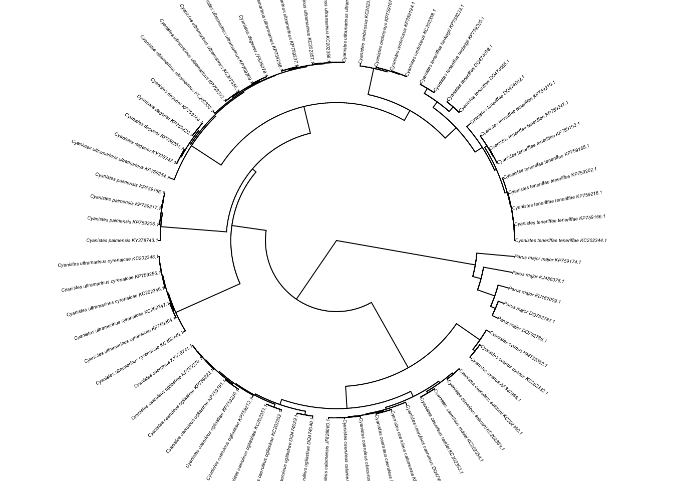

Zoom-in on different parts of the tree. With the function below you can click on parts of the tree to see a zoomed-in version.

subtreeplot(ladderize(cyanistes),cex=0.4)

Remove the outgroup (delete all Parus individuals), by creating a new tree object without all the tips belonging to the outgroup.

cyanistes_ingroup<-drop.tip(cyanistes,c("Parus_major_major_KP759174.1",
                                         "Parus_major_DQ792786.1", 
                                         "Parus_major_DQ792787.1",
                                         "Parus_major_EU167009.1", 
                                         "Parus_major_KJ456375.1"))

And we can now plot the new tree with only the ingroup to check if it worked:

par(mfrow=c(1,1))
plot(ladderize(cyanistes_ingroup),cex=0.4,no.margin=TRUE)