library(phytools)7 Ancestral area reconstruction
7.1 Reconstruct ancestral areas
Ancestral area reconstructions are statistical approaches to infer past ranges along the branches and nodes of a phylogeny, based on the geographical distribution data of the extant species (i.e., the tips). These methods are very popular in the field of historical biogeography and island biogeography, as they allow making inferences about movements between geographical regions. We will use R for this.
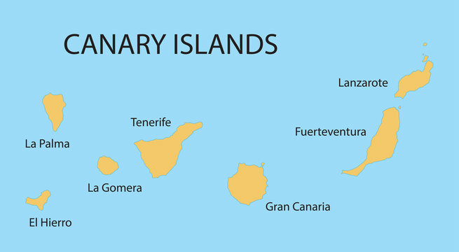
In the case of Cyanistes, we are interested in inferring how many times the Canary Islands have been colonised from the mainland. The Canary Islands are composed of 7 main islands, and some Cyanistes lineages are found on only a few islands.
Load the phytools package, which includes a function for character reconstruction.
Load table with the distribution data for all tips in the tree available in this file. Important: the names in the table must match exactly those in your tree otherwise R will not be able to match the distribution to the corresponding tip. (If they are different, change them directly in the .csv file or in your tree file)
island_data<-read.csv("data/Cyanistes_distribution.csv",header=T)View the table. It has 2 columns, one with the tip names and other with their geographical distribution.
View(island_data)Run the chunk of code below to format the data to run ancestral area reconstruction analysis.
island_d<-as.data.frame(island_data$Distribution)
taxa<-as.data.frame(island_data$Species)
islands<-as.data.frame(island_d[match(cyanistes$tip.label,taxa[,1]),])
islands<-t(islands)
islands<-as.character(islands)
names(islands)<-cyanistes$tip.label
Perform the ancestral area reconstruction, using the function make.simmap. This a popular function for reconstructing character states along a phylogeny (stochastic character mapping). It is not necessarily the best for ancestral area reconstruction, because there are more appropriate models. But for the purposes of the practical we will use it. Takes a while to run.
set.seed(3)
cyanistes_simmap<-make.simmap(cyanistes,islands,model="ER",nsim=1000)
make.simmap is sampling character histories conditioned on
the transition matrix
Q =
ElHierro Fuerteventura GranCanaria LaGomera Mainland
ElHierro -0.32321739 0.05386957 0.05386957 0.05386957 0.05386957
Fuerteventura 0.05386957 -0.32321739 0.05386957 0.05386957 0.05386957
GranCanaria 0.05386957 0.05386957 -0.32321739 0.05386957 0.05386957
LaGomera 0.05386957 0.05386957 0.05386957 -0.32321739 0.05386957
Mainland 0.05386957 0.05386957 0.05386957 0.05386957 -0.32321739
Palma 0.05386957 0.05386957 0.05386957 0.05386957 0.05386957
Tenerife 0.05386957 0.05386957 0.05386957 0.05386957 0.05386957
Palma Tenerife
ElHierro 0.05386957 0.05386957
Fuerteventura 0.05386957 0.05386957
GranCanaria 0.05386957 0.05386957
LaGomera 0.05386957 0.05386957
Mainland 0.05386957 0.05386957
Palma -0.32321739 0.05386957
Tenerife 0.05386957 -0.32321739
(estimated using likelihood);
and (mean) root node prior probabilities
pi =
ElHierro Fuerteventura GranCanaria LaGomera Mainland
0.1428571 0.1428571 0.1428571 0.1428571 0.1428571
Palma Tenerife
0.1428571 0.1428571 Done.pd<-summary(cyanistes_simmap,plot=FALSE)simmap is stochastic simulation model, which means that you may obtain different reconstructions if you run the model different times, and the reconstruction may differ between computers. By setting the “seed” (random value setting) above we ensure that the same reconstruction can be reproduced.
Using the code below, plot the tree with the ancestral areas reconstructed. The colours indicate the areas reconstructed for each branch.
par(oma=c(0,0,0,0))
cols<-setNames(palette()[1:length(unique(islands))],sort(unique(islands)))
plot(cyanistes_simmap[[1]],cols,fsize=0.8)
add.simmap.legend(colors=cols,prompt=FALSE,x=0.9*par()$usr[1],
                  y=25,fsize=0.8)
Optionally, you can also add pie charts for the reconstructed areas at tips and nodes. The pie charts on the nodes indicate the uncertainty in the biogeographical reconstruction. (the code below only works if you already plotted the tree using the code above).
nodelabels(pie=pd$ace,piecol=cols,cex=0.3)

tiplabels(pie=to.matrix(islands,sort(unique(islands))),piecol=cols,cex=0.1)
Based on this tree, can you infer how many colonisation events of the Canary Islands there have been?
Combining with Figtree to check for the node ages, can you estimate when these colonisations took place?
Do you see any evidence for back-colonisation in the cytochrome-B data? (this would be a species or clade of mainland individuals, nested within an island clade).